Surface integral of the 1st kind. Calculation of surface integrals: theory and examples. MA. Surface integrals of the second kind

Example 3.3. Calculate the work of a vector field

a = 2x 2 y i – xy 2 j

from the origin O to point A(1;1), if the movement occurs along: A) line segment; b) arcs of a parabola; V) broken line OBA, where B(1;0) (see Fig. 3.1).

Solution . A) The equation of straight line OA has the form y=x. Let x=t, then the equation of the straight line in parametric form will take the form:

x=t, y=t,

and when moving from A to B the parameter t will change from 0 to 1. Then the work done will be equal to

b) Let x=t 2 , y=t, Then

x=t 2 , y=t, 0£ t£1 .

.

V) The equation of the line (OB) is y=0 (0£ x£1); the equation of the line (BA) has the form x=1 (0 £ y£1). Then

, .

As a result, we get,

.

Comment. If in the case of two-dimensional fields the line equation is described by the equation y=y(x), and the variable x varies from a before b, then the curvilinear integral of the 2nd will be calculated by the formula:

. (3.9)

The previous example could be solved using this formula without introducing the parameter t.

Example 3.4. Calculate integral

,

where L is the arc of the parabola y=x 2 +1 from point A(0;1) to point B(2;5).

Solution . Let's make a drawing (see Fig. 3.2). From the parabola equation we get y"=2x. Since on the arc of a parabola AB variable x changes from 0 to 2, then the curvilinear integral, in accordance with formula (3.9), will take the form

4. SURFACE INTEGRALS

4.1. Surface integrals of the first kind

The surface integral of the 1st kind is a generalization of the double integral and is introduced in a similar way. Consider some surface S, smooth or piecewise smooth, and assume that the function f( x,y,z) is defined and limited on this surface. Let us divide this surface into n arbitrary parts. The area of ​​each plot is denoted by D s i. On each section we select a point with coordinates ( x i ,y i ,z i) and calculate the value of the function at each such point. After this, we create the integral sum:

.

If there is a limit of integral sums at n®¥ (in this case max D s i®0), i.e. such a limit does not depend either on the method of partitioning or on the choice of midpoints, then such a limit is called surface integral of the first kind :

. (4.1)

If the function f( x,y,z) is continuous on the surface S, then limit (4.1) exists.

If the integrand function f( x,y,z)º1, then the surface integral of the 1st kind is equal to the surface area S:

. (4.2)

Let us assume that a Cartesian coordinate system is introduced, and any straight line parallel to the axis Oz, can cross the surface S only at one point. Then the surface equation S can be written in the form

z = z(x,y)

and it is uniquely projected onto the plane xOy. As a result, the surface integral of the 1st kind can be expressed in terms of the double integral

. (4.3)

Example 4.1. Calculate integral

,

Where S– part of the conical surface z 2 =x 2 +y£2.0 z£1.

Solution. We have

Then the required integral is transformed into a double integral

Where S xy- circle x 2 +y 2 £1. That's why

.

4.2. Surface integrals of the second kind

Let a vector field be specified in some region

a = a x i + a y j + a z k

and any double-sided surface S. Let us divide the surface in some way into elementary areas D S i. On each site we choose an arbitrary point P i and compose the integral sum:

, (4.4)

Where n (P i) – normal vector to given surface at the point P i. If there is a limit to such a sum under D S i®0, then this limit is called surface integral of the 2nd kind (or flow vector field a through the surface S) and is denoted by the symbol

or ,

Where d s =n ds.

Since the unit normal vector has directional cosines as its coordinates n =(cosa, cosb, cosg). That

Thus, the calculation of surface integrals of the 2nd kind can be reduced to the calculation of surface integrals of the 1st kind. However, what Unlike surface integrals of the 1st kind, integrals of the 2nd kind depend on the choice of the side of the surface. Transition to the other side of the surface changes the direction of the normal to the surface, and, accordingly, the sign of the integral.

Consider the integral

.

Let the surface equation have the form z=j( x,y) and the positive side of this surface will be considered to be the one whose normal forms with the O axis z sharp corner. Then

cosg ds = dxdy.

Therefore, the integral under consideration can be written in the form

.

Replacing z by j( x,y), we arrive at the double integral

,

Where S xy– surface projection S to the plane xOy.

Theoretical minimum

This topic continues the discussion of curvilinear and surface integrals that began in the topic "". It is recommended that you familiarize yourself with this topic in advance. Due to the greater complexity of the topic, curvilinear and surface integrals
the second kind are considered separately. Surface integrals of the second kind are discussed here - perhaps the most complex integral operation in
analysis of functions of many variables. The plan will be completely similar to the consideration of a curvilinear integral of the second kind. Let's start with physical applications,
and then we will move on to the formal mathematical aspect.

1. Physical Applications surface integral of the second kind

Most natural way introduce a surface integral of the second kind - consider the flow of fluid through a certain surface. Let's start with a simple case:
the liquid flows along the x-axis at a constant speed. Let us select an area perpendicular to the flow and find the mass of fluid passing through
her in time. During this time, a “parallelepiped” with a height and base area of ​​. The mass of this “parallelepiped”
equal to , where is the density of the liquid.

Now let the liquid flow parallel to the plane at an angle to the x-axis, but still with a speed. The site from the previous
case we will still place it perpendicular to the abscissa axis. Over time, an inclined “parallelepiped” passes through it (see Fig. 1). Its mass
equal to . Note that introducing a unit normal vector to the site allows us to write .
A formal vector of an elementary area is introduced, the modulus of which is equal to , and its direction coincides with the direction of the vector
normal to the site. Then . This notation allows you not to worry about the direction of the fluid velocity vector with respect to
to the site.

It remains to abandon the smallness of the area through which the liquid flows, and the assumption of a constant modulus and direction of velocity. Then
the surface is divided into small parts, within which the velocity vector can be considered constant. The mass of liquid passing through the surface is
is approximately given by the sum
.
The exact formula will be obtained in the limit of dividing the surface into infinitesimal parts. The limit is a surface integral of the second kind:
.
When writing this section, a fragment was used educational material teacher of the Department of General Physics, used by him in seminar classes.

2. Definition of a surface integral of the second kind

Now about the formal construction of the integral. Due to the fact that the vector field is integrated over the surface, it makes sense to clarify on which side
surface, the integral is calculated (as when calculating the flow of a liquid: liquid flows into the surface or flows out of it). Therefore, it is especially specified
that the surface over which integration is carried out must be two-sided or orientable (i.e. the Möbius strip as a whole will not work). Surface
immediately oriented, i.e. a certain direction of the normal to the surface is selected (for example, if the integral is calculated over a sphere, then the normal can be
directed from the sphere or into the sphere). The field components are in general case functions of a point. Surface of integration
is divided into small parts, a point is selected in each part and the sum is compiled
,
where is the area of ​​the projection of the element onto the plane, is the area of ​​the projection of this element onto the plane, is the area
projection of this element onto a plane. We carry out the summation over all elements into which the surface is divided:

and go to the limit, directing the diameter of the largest partial region to zero. The limit is a surface integral of the second kind
.

Let us show how to reduce this integral to the form from step 1. To do this, you will have to make a small digression of a purely geometric nature. Let there be
plane intersecting the coordinate axes (see Fig. 2). The part of this plane located in the first octant has an area of ​​. You need to find the area
all three orthogonal projections of a given part of the plane onto coordinate planes. As is known, the projection area of ​​a figure is equal to the product of the area
the figure itself and the cosine of the angle between the plane of the figure and the plane on which it is projected (see Fig. 3). Those. need to find the angles that make
plane with coordinate planes. Angle between two planes equal to angle between their normals. The unit normal to the plane has components,
which are its direction cosines. Therefore, the angle between the plane and the plane is equal (see Fig. 2), and therefore .
The same relationship will be valid for infinitesimal areas: . And similarly.
Taking these relations into account, the integral takes the form
.
By the way, this form of recording is more visual, so we will work with it.

Reversing the direction of the normal causes the integral to change sign.

3. Calculation of the surface integral of the second kind

After reducing the integral to a form containing the direction cosines of the normal to the surface, the problem essentially reduces to writing the unit normal
with further calculation of the surface integral of the first kind. There are some specifics in these actions, so let’s look at the calculation in detail
integrals of this type.

Let's start with the case when the integration surface is given explicit equation, For example, . Then the normal vector is written as follows:
,
and the surface area element
.
As a result, the surface integral takes the following form:
, (1)
where is the region of the plane into which the integration surface is projected.

It may be that the surface of integration is correctly projected onto the plane (and given by the equation) or onto the plane
(and is given by the equation ). Then the formula by which the integral is calculated is slightly adjusted:
(2)
or
. (3)
Of course, it is not recommended to memorize such formulas: it is easy to confuse something - it is better to restore them in relation to a specific
calculation again, based on the formula for the normal vector and the area of ​​a small surface element.

There is one highlighted case when the surface is correctly projected onto all three coordinate planes, i.e. from the surface equation any variable
can be expressed unambiguously. Then the calculation is significantly simplified. Pay attention to the structure of formulas (1) - (3). In each of them there are three
terms, and one of them looks simpler than the others. When projecting a surface onto a plane, this term contains the component
fields ; when projected onto a plane, this is the term containing the component ; when projected onto a plane, this is the term
containing component. If the surface projects correctly onto any coordinate plane, then we split the integral
into three parts and design each part in the most convenient way:
.

Finally, the case of parametrically defining the surface
.
As when calculating a surface integral of the first kind, three Jacobians need to be considered:
.
The direction cosines of the normal are expressed through them:
,
surface element
.
Thus, for the integral we obtain
,
where is the range of parameter changes corresponding to the integration surface.

4. Stokes formula. Ostrogradsky-Gauss formula

The surface integral of the second kind is associated with two formulas that find various applications, including in physical applications.
Stokes formula:
,
Where ,
the surface is stretched over the contour, the traversal of the contour is consistent with the choice of the normal to the surface according to the right-hand screw rule.
Clarifications are required if the integration surface has “holes”.
Green's formula is a special case of this formula. In addition, from the Stokes formula it follows the condition for the independence of the curvilinear integral of the second
kind of from the shape of the path.

Ostrogradsky-Gauss formula.
For a vector field the formula is fulfilled

where the surface limits the volume.

The Ostrogradsky-Gauss formula has different applications. Let's look at two of them. First, it is easy to prove that the volume of a body can be calculated
according to the formula

Secondly, sometimes it is necessary to calculate a surface integral of the second kind over an open surface, which involves cumbersome calculations.
Then the surface is closed, the integral is converted to a triple one, and the integral over the added surface is subtracted (see example below).

Note. The Stokes and Ostrogradsky-Gauss formulas are more conveniently written in vector analysis using the curl and divergence of the vector field.

Examples of calculating surface integrals of the second kind

Example 1. Plane integral.. Then we get) parts of an elliptic paraboloid (external normal).

Let us rewrite the integral in the form
.
The integration surface - an elliptic paraboloid - is correctly projected only onto the plane, so we write the surface equation in the form
.
Find the unit normal vector:
.

For cases when integration occurs not over a segment of a curve, but over a bounded surface. Like curvilinear integrals, surface integrals are of the first kind and the second kind.

Surface integral of the first kind written in the form

Where f(M) = f(x,y,z) is a function of three variables, and the surface σ - area of ​​integration of this function. If f(x,y,z) is equal to unity, then the surface integral is equal to the surface area.

Imagine a fairly large sunflower with very, very small seeds. Then, from the sum of the surfaces of very, very small seeds located on the surface of a sunflower, one can calculate the surface of the sunflower - this may be a simplified interpretation of the surface integral. Why is that?

Let's move on to a more formal definition of a surface integral. Surface σ divided into n parts with areas Δ σ 1 , Δ σ 2 , ..., Δ σ n. If you select an arbitrary point on each partial surface (seed) Mi with coordinates ( ζ i, η i, ς i ,), then we can sum up

This sum is called the integral sum for the function f(M) on the surface σ . Now we will maximize the number of such small parts, and the largest diameter Δ σ i- on the contrary, reduce. If the integral sum as the largest of the diameters of the parts tends to zero (that is, as we have already noted, all the parts are very small) has a limit, then this limit is called surface integral of the first kind from function f(M) on the surface σ .

Calculation of the surface integral of the first kind

Let the surface σ given by the equation z = z(x, y) , its projection onto the plane xOy is the area Dxy, while the function z = z(x, y) and its partial derivatives are continuous in the region Dxy.

Example 1.

Where σ - part of the plane in the first octant.

Solution. Drawing:

From the equation of the plane we obtain the expression “zet”: .

Then the partial derivatives are: , and

.

Surface σ is the triangle shown in the drawing ABC, and its projection onto the plane xOy- triangle AOB, which is limited by straight lines x = 0 , y= 0 and 3 x + y= 6. Let’s move from the surface integral to the double integral and solve it:

.

The concept of a surface integral of the second kind

Before moving on to the definition of a surface integral of the second kind, it is necessary to become familiar with the concepts of sides of surfaces and oriented surfaces.

Let a smooth surface be given in space σ . Let's choose an arbitrary point on this surface M and draw the normal vector to the surface through it. Through the point M we will also carry out on the surface σ an arbitrary contour that has no common points with the surface boundary σ . Full stop M together with the normal vector, we will move along the contour so that the normal vector is constantly perpendicular to the surface σ . Upon return of the point M to the initial position, two cases are possible: the direction of the normal vector will remain the same or will change to the opposite.

If the direction of the normal vector does not change, then the surface σ called bilateral. If, when traversing the contour, the direction of the normal vector changes to the opposite, then the surface is called one-sided. Double-sided surfaces are called oriented surfaces, one-sided surfaces are called unoriented surfaces.

An example of a one-sided surface is a Möbius strip (in the picture above), which can be made from a strip of paper with one side rotated 180 degrees and then the ends glued together. And here's what's important here: for a one-sided surface the concept of a surface integral of the second kind is not introduced .

So we will consider only two-sided surfaces. Examples of two-sided surfaces are planes, spheres, ellipsoids, and paraboloids.

The positive side of a two-sided surface determines the direction of the normal vector. The opposite side of the surface is called negative. On the positive side surface is called its upper side. If the unit normal vectors make acute angles with the axis Oz, then the top side of the surface is selected z = z(x, y) , if the angles are obtuse, then the bottom side of the surface.

As in the case of the surface integral of the first kind, the surface can be divided into n parts. When formulating the concept of a surface integral of the first kind, the integral sum included the areas of each of the parts by which the values ​​of the function were multiplied f(Mi). In the case of a surface integral of the second kind, the areas of the parts themselves are not taken, but the areas of their projections onto coordinate planes . And to distinguish the function of three variables from an integral of the first kind we denote R(x,y,z) . Then the integral sum will be written as follows:

,

where Δ si- the areas of the mentioned projections of parts of the side of the surface onto the coordinate axis (for now we will assume that on the axis xOy).

With such conventions and notation, the definition of a surface integral of the second kind is similar to the definition of an integral of the first kind. Namely: a surface integral of the second kind is the limit of a given integral sum as the largest diameter of the parts of the surface under consideration tends to zero.

It is written like this:

.

In this case the function R(x,y,z) integrable over variables x And y, since parts of the surface were projected onto the plane xOy.

Similarly, we can write two other surface integrals of the second kind:

(function P(x,y,z) integrable over variables y And z yOz),

(function Q(x,y,z) integrable over variables z And x, since parts of the surface are projected onto the plane zOx).

The sum of these integrals

called general surface integral of the second kind and is designated

Calculation of the surface integral of the second kind

A surface integral of the second kind is calculated by decomposing the general surface integral of the second kind into the sum of surface integrals (see the end of the previous paragraph) and reducing each of them to a double integral.

Let us consider in detail the calculation of the integral

.

Let the surface σ given by the equation z = z(x, y) . We denote the positive side of the surface, the negative side, and the projection onto the plane xOy - Dxy.

Thus, we obtain a formula for calculating the surface integral of the second kind:

If selected negative side surface, then the sign of the integral changes:

The other two separate integrals - terms of the general one - are calculated similarly:

Example 2.

,

Where σ - the upper side of a part of the plane, cut off by planes y= 0 and y= 4 and located in the first octant.

Solution. The drawing is in the picture above. By definition, we obtain the sum of three double integrals:

The second integral is equal to zero, since the plane σ parallel to the axis Oy. Therefore, we find the first and third integrals:

All that remains is to add up all the individual integrals and obtain the general surface integral of the second kind:

.

If you need to calculate a surface integral of the second kind over a closed surface, you can go to triple integral, using the Ostrogradsky formula. Then, if the functions P(x,y,z) , Q(x,y,z) And R(x,y,z) and their partial derivatives , , are continuous functions in the domain W, which is bounded by a closed surface σ , then when integrating over the outside of the surface, the equality

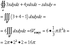
Example 3. Calculate surface integral of the second kind

,

Where σ - the outer side of the surface of a cone formed by a surface and a plane z = 2 .

Solution. This surface is the surface of a cone with a radius R= 2 and height h= 2 . This is a closed surface, so you can use Ostrogradsky's formula. Because P = 3x , Q = 4y , R = −z, then the partial derivatives , , .

We move on to the triple integral, which we solve:

More examples on calculating surface integrals

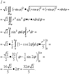
Example 4. Calculate surface integral of the first kind

Where σ - lateral surface of the cone at .

Solution. Since the partial derivatives , , 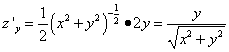That

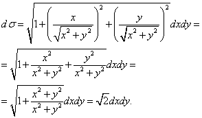
We reduce this surface integral to a double one:

Projection of a surface onto a plane xOy is a circle with center at the origin and radius R= 2, therefore, when calculating the double integral, we move to the polar coordinate system. To do this, let's change the variables:

We obtain the following integral, which we finally solve:

Example 5. Calculate surface integral of the second kind

,

Where σ - the upper part of the triangle formed by the intersection of the plane with the coordinate planes.

Solution. Let us divide this surface integral by the sum of two integrals

, Where

.

To calculate the integral I1 σ to the plane yOz. The projection is a triangle OCB, which is on the plane yOz limit straight lines or, y= 0 and z= 0 . From the equation of the plane is derived. Therefore we can calculate the integral I1 :

To calculate the integral I2 , let's construct a surface projection σ to the plane zOx. The projection is a triangle AOC, which is bounded by straight lines or , x= 0 and z= 0 . We calculate:

We add the two resulting integrals and finally obtain this surface integral:

.

Example 6. Calculate surface integral of the second kind

,

Where σ - the outer surface of a pyramid formed by a plane and coordinate planes.

If, when determining the length of a curve, it was given as the limit of a broken line inscribed in a given curve as the length of its largest segment tends to zero, then an attempt to extend this definition to the area of ​​a curved surface can lead to a contradiction (Schwartz’s example: one can consider a sequence of polyhedra inscribed in a cylinder, for which the greatest distance between points on any face tends to zero, and the area tends to infinity). Therefore, we determine the surface area in a different way. Let us consider an open surface S, bounded by a contour L, and divide it by some curves into parts S1, S2,…, Sn. Let us select a point Mi in each part and project this part onto a tangent plane to the surface passing through this point. We get in projection flat figure with area Ti. Let us call ρ the greatest distance between two points of any part of the surface S.

Definition 12.1. Let us call the surface area S the limit of the sum of areas Ti at

Surface integral of the first kind.

Let's consider some surface S, bounded by a contour L, and divide it into parts S1, S2,..., Sp (we will also denote the area of ​​each part as Sp). Let the value of the function f(x, y, z) be specified at each point of this surface. Let us select a point Mi (xi, yi, zi) in each part Si and compose the integral sum

. (12.2)

Definition 12.2. If there is a finite limit for the integral sum (12.2), independent of the method of dividing the surface into parts and the choice of points Mi, then it is called a surface integral of the first kind of the function f(M) = f(x, y, z) over the surface S and is denoted

Comment. A surface integral of the 1st kind has the usual properties of integrals (linearity, summation of integrals of a given function over separate parts surface under consideration, etc.).

Geometric and physical meaning of a surface integral of the 1st kind.

If the integrand function f(M) ≡ 1, then from Definition 12.2 it follows that is equal to the area of ​​the surface S under consideration.

Calculation of surface integral of the 1st kind.

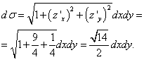
Let us restrict ourselves to the case when the surface S is specified explicitly, that is, by an equation of the form z = φ(x, y). Moreover, from the definition of surface area it follows that

Si = , where Δσi is the area of ​​projection of Si onto the Oxy plane, and γi is the angle between the Oz axis and the normal to the surface S at point Mi. It is known that

,

where (xi, yi, zi) are the coordinates of point Mi. Therefore,

Substituting this expression into formula (12.2), we obtain that

,

where the summation on the right is carried out over the region Ω of the Oxy plane, which is the projection of the surface S onto this plane (Fig. 1).

In this case, on the right side, an integral sum is obtained for a function of two variables over a flat region, which in the limit at gives a double integral. Thus, a formula has been obtained that allows one to reduce the calculation of a surface integral of the 1st kind to the calculation of a double integral.