Model of a “predator-prey” situation. Predator-prey equilibrium Mathematical model conservative predator prey
Kolmogorov's model makes one significant assumption: since it is assumed that this means that there are mechanisms in the prey population that regulate their numbers even in the absence of predators.
Unfortunately, such a formulation of the model does not allow answering the question around which Lately There is a lot of debate, which we already mentioned at the beginning of the chapter: how can a population of predators exert a regulatory influence on a population of prey so that the entire system is sustainable? Therefore, we will return to model (2.1), in which self-regulation mechanisms (for example, regulation through intraspecific competition) are absent in the prey population (as well as in the predator population); therefore, the only mechanism for regulating the numbers of species included in a community is the trophic relationship between predators and prey.
Here (so, unlike the previous model, Naturally, solutions (2.1) depend on the specific type of trophic function which, in turn, is determined by the nature of predation, i.e., the trophic strategy of the predator and defensive strategy victims. The following properties are common to all these functions (see Fig. I):
System (2.1) has one nontrivial stationary point, the coordinates of which are determined from the equations
![]()
under natural limitation.
There is one more stationary point (0, 0), corresponding to the trivial equilibrium. It is easy to show that this point is a saddle, and the separatrices are the coordinate axes.
The characteristic equation for a point has the form
![]()
Obviously, for the classical Volterra model .
Therefore, the value of f can be considered as a measure of the deviation of the model under consideration from the Volterra model.
![]()
a stationary point is the focus, and oscillations appear in the system; when the opposite inequality is satisfied, there is a node, and there are no oscillations in the system. The stability of this equilibrium state is determined by the condition
i.e., it significantly depends on the type of trophic function of the predator.
Condition (5.5) can be interpreted as follows: for the stability of the nontrivial equilibrium of the predator-prey system (and thus for the existence of this system), it is sufficient that in the vicinity of this state the relative proportion of prey consumed by the predator increases with the increase in the number of prey. Indeed, the proportion of prey (out of their total number) consumed by a predator is described by a differentiable function, the condition for which to increase (positive derivative) looks like
![]()
The last condition taken at the point is nothing more than condition (5.5) for the stability of equilibrium. With continuity, it must also be fulfilled in a certain neighborhood of the point. Thus, if the number of victims in this neighborhood, then
Let now the trophic function V have the form shown in Fig. 11, a (characteristic of invertebrates). It can be shown that for all finite values (since it is convex upward)
that is, for any value of the stationary number of victims, inequality (5.5) is not satisfied.
This means that in a system with this type of trophic function there is no stable non-trivial equilibrium. Several outcomes are possible: either the numbers of both prey and predator increase indefinitely, or (when the trajectory passes near one of the coordinate axes) due to random reasons the number of prey or the number of predators will become zero. If the prey dies, after some time the predator will also die, but if the predator dies first, then the number of the prey will begin to increase exponentially. The third option - the emergence of a stable limit cycle - is impossible, which is easily proven.
In fact, the expression

in the positive quadrant is always positive, unless it has the form shown in Fig. 11, a. Then, according to the Dulac criterion, there are no closed trajectories in this region and a stable limit cycle cannot exist.
So, we can conclude: if the trophic function has the form shown in Fig. 11, and then the predator cannot be a regulator that ensures the stability of the prey population and thereby the stability of the entire system as a whole. The system can be stable only if the prey population has its own internal regulatory mechanisms, for example, intraspecific competition or epizootics. This regulation option has already been discussed in §§ 3, 4.
It was previously noted that this type of trophic function is characteristic of insect predators, whose “victims” are also usually insects. On the other hand, observations of the dynamics of many natural communities"predator-prey" types, which include insect species, show that they are characterized by oscillations of very large amplitude and of a very specific type.
Usually, after a more or less gradual increase in numbers (which can occur either monotonically or in the form of oscillations with increasing amplitude), a sharp drop occurs (Fig. 14), and then the picture repeats. Apparently, this nature of the dynamics of the numbers of insect species can be explained by the instability of this system at low and medium numbers and the action of powerful intrapopulation regulators of numbers at large numbers.

Rice. 14. Population dynamics of the Australian psyllid Cardiaspina albitextura feeding on eucalyptus trees. (From the article: Clark L. R. The population dynamics of Cardiaspina albitextura.-Austr. J. Zool., 1964, 12, No. 3, p. 362-380.)
If the “predator-prey” system includes species capable of sufficient challenging behavior(for example, predators are capable of learning or victims are able to find shelter), then in such a system the existence of a stable non-trivial equilibrium is possible. This statement is proven quite simply.
In fact, the trophic function should then have the form shown in Fig. 11, c. The point on this graph is the tangency point of the straight line drawn from the origin of the trophic function graph. Obviously, at this point the function has a maximum. It is also easy to show that condition (5.5) is satisfied for all. Consequently, a nontrivial equilibrium in which the number of victims is smaller will be asymptotically stable
However, we cannot say anything about how large the region of stability of this equilibrium is. For example, if there is an unstable limit cycle, then this region must lie inside the cycle. Or another option: the nontrivial equilibrium (5.2) is unstable, but there is a stable limit cycle; in this case we can also talk about the stability of the predator-prey system. Since expression (5.7) when choosing a trophic function like Fig. 11, in can change sign when changing at , then the Dulac criterion does not work here and the question of the existence of limit cycles remains open.

PA88 system, which simultaneously predicts the likelihood of more than 100 pharmacological effects and mechanisms of action of a substance based on its structural formula. The effectiveness of this approach to planning screening is about 800%, and the accuracy of the computer forecast is 300% higher than the prediction of experts.
So, one of the constructive tools for obtaining new knowledge and solutions in medicine is the method of mathematical modeling. The process of mathematization of medicine is a frequent manifestation of the interpenetration of scientific knowledge, increasing the efficiency of treatment and preventive work.
4. Mathematical model “predator-prey”
For the first time in biology, a mathematical model of periodic changes in the number of antagonistic animal species was proposed by the Italian mathematician V. Volterra and his colleagues. The model proposed by Volterra was a development of the idea outlined in 1924 by A. Lottka in the book “Elements of Physical Biology”. Therefore, this classical mathematical model is known as the “Lottky-Volterra” model.
Although in nature the relationships of antagonistic species are more complex than in a model, they are nevertheless a good teaching model on which to study the basic ideas of mathematical modeling.
So, the problem: in some ecologically closed area there live two species of animals (for example, lynxes and hares). Hares (prey) feed on plant food, which is always available in sufficient quantity (this model does not take into account limited resources plant food). Lynxes (predators) can only eat hares. It is necessary to determine how the numbers of prey and predators will change over time in such an ecological system. If the prey population increases, the probability of encounters between predators and prey increases, and, accordingly, after a certain time delay, the predator population increases. This one is enough simple model quite adequately describes the interaction between real populations of predators and prey in nature.
Now let's get started drawing up differential equations. About
let's denote the number of prey by N, and the number of predators by M. The numbers N and M are functions of time t. In our model we take into account the following factors:
a) natural reproduction of victims; b) natural death of victims;
c) destruction of victims by eating them by predators; d) natural extinction of predators;
e) an increase in the number of predators due to reproduction in the presence of food.
Because we're talking about about the mathematical model, the task is to obtain equations that would include all the intended factors and that would describe the dynamics, that is, the change in the number of predators and prey over time.
Let the number of prey and predators change by ∆N and ∆M over some time t. The change in the number of victims ∆N over time ∆t is determined, firstly, by the increase as a result of natural reproduction (which is proportional to the available number of victims):
where B is the proportionality coefficient characterizing the rate of natural extinction of victims.
The derivation of the equation describing the decrease in the number of prey due to their consumption by predators is based on the idea that the more often they are encountered, the faster the number of prey decreases. It is also clear that the frequency of encounters between predators and prey is proportional to both the number of victims and the number of predators, then
Dividing the left and right side equation (4) on ∆t and passing to the limit at ∆t→0, we obtain differential equation first order:
In order to solve this equation, you need to know how the number of predators (M) changes over time. The change in the number of predators (∆M) is determined by an increase due to natural reproduction in the presence of sufficient food (M 1 = Q∙N∙M∙∆t) and a decrease due to the natural extinction of predators (M 2 = - P∙M∙∆ t):
M = Q∙N∙M∙∆t - P∙M∙∆t |
From equation (6) we can obtain the differential equation:
Differential equations (5) and (7) represent a mathematical “predator-prey” model. It is enough to determine the values of the coefficient

ents A, B, C, Q, P and a mathematical model can be used to solve the problem.
Checking and adjusting the mathematical model. In this laboratory
In addition to calculating the most complete mathematical model (equations 5 and 7), it is proposed to study simpler ones in which something is not taken into account.
Having considered the five levels of complexity of the mathematical model, you can “feel” the stage of checking and adjusting the model.
1st level – in the model, only their natural reproduction is taken into account for “preys”, there are no “predators”;
Level 2 – the model takes into account the natural extinction of “preys”, there are no “predators”;
Level 3 – the model takes into account the natural reproduction of “victims”
And extinction, no “predators”;
4th level – the model takes into account the natural reproduction of “victims”
And extinction, as well as being eaten by “predators”, but the number of “predators” remains unchanged;
Level 5 – the model takes into account all the factors discussed.
So, we have the following system of differential equations:
where M is the number of “predators”; N – number of “victims”;
t – current time;
A – rate of reproduction of “victims”; C – frequency of predator-prey encounters; B – rate of extinction of “victims”;
Q – reproduction of “predators”;
P – extinction of “predators”.
1st level: M = 0, B = 0; 2nd level: M = 0, A = 0; 3rd level: M = 0; 4th level: Q = 0, P = 0;
Level 5: complete system of equations.
Substituting the values of the coefficients into each level, we will obtain different solutions, for example:
For the 3rd level the value of the coefficient M=0, then

solving the equation we get
Likewise for levels 1 and 2. As for the 4th and 5th levels, here it is necessary to solve the system of equations using the Runge-Kutta method. As a result, we obtain a solution to mathematical models of these levels.
II. STUDENTS' WORK DURING PRACTICAL LESSONS
Exercise 1 . Oral speech control and correction of mastering the theoretical material of the lesson. Passing admission to classes.
Task 2. Carrying out laboratory work, discussing the results obtained, writing notes.
Completing of the work
1. From the computer desktop, call the “Lab. No. 6” program by double-clicking on the corresponding shortcut with the left mouse button.
2. Double-click the left mouse button on the "PREDATOR" shortcut.
3. Select the "PRED" shortcut and repeat the program call with the left mouse button (by double-clicking).
4. After the title screen, press "ENTER".
5. Modeling starts with 1st level.
6. Enter the year from which the model will be analyzed: for example, 2000
7. Select time intervals, for example, within 40 years, after 1 year (then after 4 years).
2nd level: B = 0.05; N0 = 200;
3rd level: A = 0.02; B = 0.05; N = 200;
4th level: A = 0.01; B = 0.002; C = 0.01; N0 = 200; M = 40; 5th level: A = 1; B = 0.5; C = 0.02; Q = 0.002; P = 0.3; N0 = 200;
9. Prepare a written report on the work, which should contain equations, graphs, results of calculating the characteristics of the model, conclusions on the work done.
Task 3. Monitoring the final level of knowledge:
a) oral report for completed work laboratory work; b) solving situational problems; c) computer testing.
Task 4. Assignment for the next lesson: section and topic of the lesson, coordination of topics for abstract reports (volume of the report 2-3 pages, time limit 5-7 minutes).
Adaptations developed by prey to counteract predators contribute to the development of mechanisms for predators to overcome these adaptations. The long-term coexistence of predators and prey leads to the formation of a system of interaction in which both groups are stably preserved in the study area. Violation of such a system often leads to negative environmental consequences.
The negative impact of disruption of coevolutionary relationships is observed during the introduction of species. In particular, goats and rabbits, introduced into Australia, do not have effective mechanisms for regulating their numbers on this continent, which leads to the destruction of natural ecosystems.
Mathematical model
Let's say that two types of animals live in a certain area: rabbits (eating plants) and foxes (eating rabbits). Let the number of rabbits , number of foxes . Using the Malthus Model with the necessary amendments taking into account the eating of rabbits by foxes, we arrive at next system, bearing the name of Volterra's model - Trays:
\begin(cases) \dot x=(\alpha -c y)x;\\
\dot y=(-\beta+d x) y. \end(cases)
Model Behavior
The group lifestyle of predators and their prey radically changes the behavior of the model and gives it increased stability.
Rationale: Group living reduces the frequency of chance encounters between predators and potential prey, which is confirmed by observations of the population dynamics of lions and wildebeest in the Serengeti Park.
Story
Model of coexistence of two biological species(populations) of the “predator-prey” type is also called the Volterra-Lotka model.
see also
Write a review of the article "Predator-prey system"
Notes
Literature
- V. Volterra, Mathematical theory struggle for existence. Per. from French O. N. Bondarenko. Under the editorship and afterword by Yu. M. Svirezhev. M.: Nauka, 1976. 287 p. ISBN 5-93972-312-8
- A. D. Bazykin, Mathematical biophysics of interacting populations. M.: Nauka, 1985. 181 p.
- A. D. Bazykin, Yu. A. Kuznetsov, A. I. Khibnik, Portraits of bifurcations (Bifurcation diagrams of dynamic systems on a plane) / Series “New in life, science, technology. Mathematics, cybernetics" - M.: Znanie, 1989. 48 p.
- P. V. Turchin,
Links
An excerpt characterizing the “predator-prey” system
“Charmant, charmant, [Lovely, charming,” said Prince Vasily.“C"est la route de Varsovie peut être, [This is the Warsaw road, maybe.] - Prince Hippolyte said loudly and unexpectedly. Everyone looked back at him, not understanding what he wanted to say by this. Prince Hippolyte also looked back with cheerful surprise around him. He, like others, did not understand what the words he said meant. During his diplomatic career I noticed more than once that the words suddenly spoken in this way turned out to be very witty, and just in case, he said these words, the first ones that came to his tongue. “Maybe it will work out very well,” he thought, “and if it doesn’t work out, they will be able to arrange it there.” Indeed, while an awkward silence reigned, that insufficiently patriotic face entered, whom Anna Pavlovna was waiting for to address, and she, smiling and shaking her finger at Hippolyte, invited Prince Vasily to the table, and, presenting him with two candles and a manuscript, asked him to begin . Everything fell silent.
- Most merciful Emperor! - Prince Vasily declared sternly and looked around the audience, as if asking if anyone had anything to say against this. But no one said anything. “The Mother See of Moscow, New Jerusalem, receives its Christ,” he suddenly emphasized his words, “like a mother into the arms of her zealous sons, and through the emerging darkness, seeing the brilliant glory of your power, sings in delight: “Hosanna, blessed is he who comes.” ! – Prince Vasily said these last words in a crying voice.
Bilibin examined his nails carefully, and many, apparently, were timid, as if asking what was their fault? Anna Pavlovna repeated in a whisper forward, like an old woman praying for communion: “Let the impudent and insolent Goliath…” she whispered.
Prince Vasily continued:
- “Let the daring and arrogant Goliath from the borders of France carry to the edges of Russia deadly horrors; meek faith, this sling of the Russian David, will suddenly strike down the head of his bloodthirsty pride. This image of St. Sergius, the ancient zealot for the good of our fatherland, is brought to your to the imperial majesty. I am sick because my weakening strength prevents me from enjoying your most kind contemplation. I send warm prayers to heaven, that the Almighty may magnify the race of the righteous and fulfill your Majesty’s good wishes.”
– Quelle force! Quel style! [What power! What a syllable!] - praise was heard to the reader and writer. Inspired by this speech, Anna Pavlovna’s guests talked for a long time about the situation of the fatherland and made various assumptions about the outcome of the battle, which was to be fought the other day.
“Vous verrez, [You will see.],” said Anna Pavlovna, “that tomorrow, on the sovereign’s birthday, we will receive news.” I have a good feeling.
Anna Pavlovna's premonition really came true. The next day, during a prayer service in the palace on the occasion of the sovereign's birthday, Prince Volkonsky was called from the church and received an envelope from Prince Kutuzov. This was a report from Kutuzov, written on the day of the battle from Tatarinova. Kutuzov wrote that the Russians did not retreat a single step, that the French lost much more than we did, that he was reporting in a hurry from the battlefield, without having yet managed to collect the latest information. Therefore, it was a victory. And immediately, without leaving the temple, gratitude was given to the creator for his help and for the victory.
Anna Pavlovna's premonition was justified, and a joyfully festive mood reigned in the city all morning. Everyone recognized the victory as complete, and some were already talking about the capture of Napoleon himself, his deposition and the election of a new head for France.
Far from business and among the conditions of court life, it is very difficult for events to be reflected in all their fullness and force. Involuntarily, general events are grouped around one particular case. So now the main joy of the courtiers was as much in the fact that we had won as in the fact that the news of this victory fell precisely on the sovereign’s birthday. It was like a successful surprise. Kutuzov’s news also spoke about Russian losses, and Tuchkov, Bagration, and Kutaisov were named among them. Also, the sad side of the event involuntarily in the local St. Petersburg world was grouped around one event - the death of Kutaisov. Everyone knew him, the sovereign loved him, he was young and interesting. On this day everyone met with the words:
- How amazing it happened. At the very prayer service. And what a loss for the Kutais! Oh, what a pity!
– What did I tell you about Kutuzov? - Prince Vasily now spoke with the pride of a prophet. “I always said that he alone is capable of defeating Napoleon.”
But the next day there was no news from the army, and the general voice became alarming. The courtiers suffered for the suffering of the unknown in which the sovereign was.
- What is the position of the sovereign! - the courtiers said and no longer extolled him as the day before, but now condemned Kutuzov, former cause the sovereign's worries. On this day, Prince Vasily no longer boasted about his protege Kutuzov, but remained silent when it came to the commander-in-chief. In addition, by the evening of this day, everything seemed to come together in order to plunge the residents of St. Petersburg into alarm and worry: another terrible news was added. Countess Elena Bezukhova died suddenly from this terrible disease, which was so pleasant to pronounce. Officially, in large societies, everyone said that Countess Bezukhova died from a terrible attack of angine pectorale [chest sore throat], but in intimate circles they told details about how le medecin intime de la Reine d "Espagne [the Queen's physician of Spain] prescribed Helen small doses some kind of medicine to produce a certain effect; but how Helen, tormented by the fact that the old count suspected her, and by the fact that the husband to whom she wrote (that unfortunate depraved Pierre) did not answer her, suddenly took a huge dose of the medicine prescribed for her and died in agony before they could give help. They said that Prince Vasily and the old count took on the Italian, but the Italian showed such notes from the unfortunate deceased that he was immediately released.
COMPUTER MODEL “PREDATOR-VICTIM”
Kazachkov Igor Alekseevich 1, Guseva Elena Nikolaevna 2
1 Magnitogorsk State Technical University them. G.I. Nosova, Institute of Construction, Architecture and Art, 5th year student
2 Magnitogorsk State Technical University named after. G.I. Nosova, Institute of Energy and Automated Systems, Candidate of Pedagogical Sciences, Associate Professor of the Department of Business Informatics and Information Technologies
annotation
This article is devoted to an overview of the “predator-prey” computer model. The conducted research suggests that environmental modeling plays a huge role in environmental research. This issue is multifaceted.
COMPUTER MODEL "PREDATOR-VICTIM"
Kazatchkov Igor Alekseevich 1, Guseva Elena Nikolaevna 2
1 Nosov Magnitogorsk State Technical University, Civil Engineering, Architecture and Arts Institute, student of the 5th course
2 Nosov Magnitogorsk State Technical University, Power Engineering and Automated Systems Institute, PhD in Pedagogical Science, Associate Professor of the Business Computer Science and Information Technologies Department
Abstract
This article provides an overview of the computer model "predator-victim". The study suggests that environmental simulation plays a huge role in the study of the environment. This problem is multifaceted.
Ecological modeling is used to study our environment. Mathematical models are used in cases where there is no natural environment and no natural objects, it helps to predict the impact various factors to the object under study. This method takes on the functions of checking, constructing and interpreting the results obtained. Based on such forms, environmental modeling deals with the assessment of changes in the environment around us.
Currently, such forms are used to study the environment around us, and when it is necessary to study any of its areas, mathematical modeling is used. This model makes it possible to predict the influence of certain factors on the object of study. At one time, the “predator-prey” type was proposed by such scientists as: T. Malthus (Malthus 1798, Malthus 1905), Verhulst (Verhulst 1838), Pearl (Pearl 1927, 1930), as well as A. Lotka (Lotka 1925, 1927 ) and V. Volterra (Volterra 1926). These models reproduce the periodic oscillatory regime that arises as a result of interspecific interactions in nature.
One of the main methods of cognition is modeling. In addition to the fact that it can predict changes occurring in environment, also helps to find the optimal way to solve the problem. Mathematical models have been used in ecology for a long time in order to establish patterns and trends in the development of populations, and help highlight the essence of observations. The layout can serve as a sample behavior, object.
When recreating objects in mathematical biology, predictions of various systems are used, special individualities of biosystems are provided for: the internal structure of the individual, life support conditions, constancy ecological systems, thanks to which the vital activity of systems is preserved.
The advent of computer modeling has significantly advanced the frontier of research capabilities. The possibility of multilateral implementation of difficult forms that do not allow analytical study has arisen; newest directions, and also simulation modeling.
Let's consider what a modeling object is. “The object is a closed habitat where interaction between two biological populations occurs: predators and prey. The process of growth, extinction and reproduction occurs directly on the surface of the habitat. The prey feeds on the resources that are present in the environment, while the predators feed on the prey. In this case, nutritional resources can be either renewable or non-renewable.
In 1931, Vito Volterra derived the following laws of the predator-prey relationship.
The law of the periodic cycle - the process of destruction of prey by a predator often leads to periodic fluctuations in the population size of both species, depending only on the growth rate of carnivores and herbivores, and on the initial ratio of their numbers.
Law of Conservation of Averages - The average abundance of each species is constant, regardless of the initial level, provided that the specific rates of population increase, as well as the efficiency of predation, are constant.
The law of violation of average values - when both species are reduced in proportion to their number, the average population size of the prey increases, and that of predators decreases.
The predator-prey model is a special relationship between a predator and its prey, as a result of which both benefit. The healthiest and most adapted individuals to the environmental conditions survive, i.e. all this happens thanks to natural selection. In an environment where there is no opportunity for reproduction, the predator will sooner or later destroy the population of the prey, as a result of which it itself will become extinct.”
There are many living organisms on earth that, under favorable conditions, increase the number of relatives to huge scale. This ability is called: the biotic potential of a species, i.e. an increase in the number of a species over a certain period of time. Each species has its own biotic potential, for example large species organisms in a year can increase by only 1.1 times, in turn, organisms of smaller species, such as crustaceans, etc. can increase their appearance up to 1030 times, but bacteria are still more. In any of these cases, the population will grow exponentially.
Exponential growth in numbers is called geometric progression population growth. This ability can be observed in the laboratory in bacteria and yeast. In non-laboratory conditions, exponential growth can be seen in the example of locusts or in other types of insects. Such an increase in the number of species can be observed in those places where it has practically no enemies, and there is more than enough food. Eventually an increase in species, after numbers had increased for a short period of time, population growth began to decline.
Let's consider a computer model of mammalian reproduction using the Lotka-Volterra model as an example. Let In a certain area, two types of animals live: deer and wolves. Mathematical model of population changes in the model Trays-Volterra:
The initial number of victims is xn, the number of predators is yn.
Model parameters:
P1 – probability of meeting with a predator,
P2 – coefficient of growth of predators at the expense of prey,
d – predator mortality rate,
a – coefficient of increase in the number of victims.
In the training task, the following values were set: the number of deer was 500, the number of wolves was 10, the growth rate of deer was 0.02, the growth rate of wolves was 0.1, the probability of meeting a predator was 0.0026, the growth rate of predators at the expense of prey was 0 ,000056. The data is calculated for 203 years.
We explore the influence the coefficient of increase in victims for the development of two populations, the remaining parameters will be left unchanged. In Scheme 1, an increase in the number of prey is observed and then, with some delay, an increase in predators is observed. Then the predators knock out the victims, the number of victims drops sharply and, following it, the number of predators decreases (Fig. 1).

Figure 1. Population size with low birth rates among victims
Let's analyze the change in the model by increasing the victim's birth rate a=0.06. In Diagram 2 we see a cyclical oscillatory process leading to an increase in the numbers of both populations over time (Fig. 2).

Figure 2. Population size at average birth rate of victims
Let's consider how population dynamics will change when high value the victim's birth rate is a=1.13. In Fig. 3 there is a sharp increase in the numbers of both populations, followed by extinction of both prey and predator. This occurs due to the fact that the population of prey has increased to such an extent that resources have begun to run out, resulting in the extinction of the prey. The extinction of predators occurs due to the fact that the number of prey has decreased and the predators have run out of resources to survive.
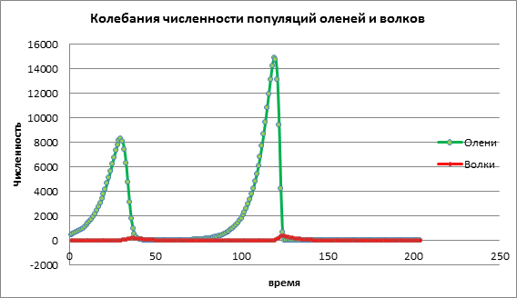
Figure 3. Population size with high birth rates among victims
Based on the analysis of computer experiment data, we can conclude that computer modeling allows us to predict population sizes and study the influence various factors on population dynamics. In the above example, we examined the predator-prey model, the influence of the birth rate of prey on the number of deer and wolves. A small increase in the prey population leads to a small increase in prey, which after a certain period is destroyed by predators. A moderate increase in the prey population leads to an increase in the size of both populations. A high increase in the prey population first leads to a rapid increase in the prey population, this affects the increase in the growth of predators, but then the multiplied predators quickly destroy the deer population. As a result, both species become extinct.
Models of interaction of two types
Volterra's hypotheses. Analogies with chemical kinetics. Volterra models of interactions. Classification of types of interactions Competition. Predator-prey. Generalized models of species interactions . Kolmogorov model. MacArthur's model of interaction between two insect species. Parametric and phase portraits of the Bazykin system.
The founder of the modern mathematical theory of populations is rightly considered the Italian mathematician Vito Volterra, who developed the mathematical theory of biological communities, the apparatus of which is differential and integro-differential equations.(Vito Volterra. Lecons sur la Theorie Mathematique de la Lutte pour la Vie. Paris, 1931). In subsequent decades, population dynamics developed mainly in line with the ideas expressed in this book. The Russian translation of Volterra’s book was published in 1976 under the title: “The Mathematical Theory of the Struggle for Existence” with an afterword by Yu.M. Svirezhev, which examines the history of the development of mathematical ecology in the period 1931–1976.
Volterra's book is written the way books on mathematics are written. It first formulates some assumptions about the mathematical objects that are supposed to be studied, and then conducts a mathematical study of the properties of these objects.
The systems studied by Volterra consist of two or more types. In some cases, the supply of food used is considered. The equations describing the interaction of these types are based on the following concepts.
Volterra's hypotheses
1. Food is either available in unlimited quantities, or its supply is strictly regulated over time.
2. Individuals of each species die off in such a way that a constant proportion of existing individuals die per unit time.
3. Predatory species eat victims, and per unit time the number of eaten victims is always proportional to the probability of meeting individuals of these two species, i.e. the product of the number of predators and the number of prey.
4. If there is food in limited quantities and several species that are able to consume it, then the share of food consumed by a species per unit time is proportional to the number of individuals of this species, taken with a certain coefficient depending on the species (models of interspecific competition).
5. If a species feeds on food available in unlimited quantities, the increase in the number of the species per unit time is proportional to the number of the species.
6. If a species feeds on food available in limited quantities, then its reproduction is regulated by the rate of food consumption, i.e. per unit time, the increase is proportional to the amount of food eaten.
Analogies with chemical kinetics
These hypotheses have close parallels with chemical kinetics. In the equations of population dynamics, as in the equations of chemical kinetics, the “collision principle” is used, when the reaction rate is proportional to the product of the concentrations of the reacting components.
Indeed, according to Volterra’s hypotheses, the speed process The extinction of each species is proportional to the number of the species. In chemical kinetics, this corresponds to a monomolecular reaction of the decomposition of a certain substance, and in a mathematical model, it corresponds to negative linear terms on the right sides of the equations.
According to the concepts of chemical kinetics, the rate of the bimolecular reaction of interaction between two substances is proportional to the probability of collision of these substances, i.e. the product of their concentration. In the same way, in accordance with Volterra’s hypotheses, the rate of reproduction of predators (death of prey) is proportional to the probability of encounters between predator and prey individuals, i.e. the product of their numbers. In both cases, bilinear terms appear in the model system on the right-hand sides of the corresponding equations.
Finally, the linear positive terms on the right-hand sides of the Volterra equations, corresponding to the growth of populations under unlimited conditions, correspond to the autocatalytic terms chemical reactions. This similarity of equations in chemical and environmental models allows us to apply the same research methods for mathematical modeling of population kinetics as for systems of chemical reactions.
Classification of types of interactions
In accordance with Volterra's hypotheses, the interaction of two species, the numbers of which x 1 and x 2 can be described by the equations:
(9.1)
Here are the parameters a i - constants of the species’ own growth rate, c i‑ constants of self-limitation of numbers (intraspecific competition), b ij- species interaction constants, (i, j= 1,2). The signs of these coefficients determine the type of interaction.
In the biological literature, interactions are usually classified according to the mechanisms involved. The diversity here is enormous: various trophic interactions, chemical interactions existing between bacteria and planktonic algae, interactions of fungi with other organisms, succession plant organisms related in particular to competition for sunlight and with the evolution of soils, etc. This classification seems vast.
E . Odum, taking into account the models proposed by V. Volterra, proposed a classification not by mechanisms, but by results. According to this classification, relationships should be assessed as positive, negative or neutral depending on whether the abundance of one species increases, decreases or remains unchanged in the presence of another species. Then the main types of interactions can be presented in table form.
TYPES OF INTERACTION OF SPECIES
|
SYMBIOSIS |
b 12 ,b 21 >0 |
||
|
COMMENSALISM |
b 12 ,>0, b 21 =0 |
||
|
PREDATOR-VICTIM |
b 12 ,>0, b 21 <0 |
||
|
AMENSALISM |
b 12 ,=0, b 21 <0 |
||
|
COMPETITION |
b 12 , b 21 <0 |
||
|
NEUTRALISM |
b 12 , b 21 =0 |
The last column shows the signs of the interaction coefficients from system (9.1)
Let's look at the main types of interactions
COMPETITION EQUATIONS:
As we saw in Lecture 6, the competition equations are:
 (9.2)
(9.2)
Stationary system solutions:
(1).
![]()
The origin of coordinates, for any system parameters, is an unstable node.
(2).
![]() (9.3)
(9.3)
C stationary state (9.3) is a saddle at a 1 >b 12 /With 2 and
stable node at a 1 12 /s 2 . This condition means that a species becomes extinct if its own growth rate is less than a certain critical value.
(3).
![]() (9.4)
(9.4)
C stationary solution (9.4)¾ saddle at a 2 >b 21 /c 1 and a stable node at a 2< b 21 /c 1
(4).
![]() (9.5)
(9.5)
Stationary state (9.5) characterizes the coexistence of two competing species and represents a stable node if the relation is satisfied:
![]()
This implies the inequality:
b 12
b 21
allowing us to formulate the condition for the coexistence of species:
The product of the coefficients of inter-population interaction is less than the product of coefficients within the population interaction.
Indeed, let the natural growth rates of the two species under considerationa 1 , a 2 are the same. Then the necessary condition for stability will be
c 2 > b 12 ,c 1 > b 21 .
These inequalities show that an increase in the size of one competitor suppresses its own growth more than the growth of another competitor. If the numbers of both species are limited, partially or completely, by different resources, the above inequalities are valid. If both species have exactly the same needs, then one of them will be more viable and will displace its competitor.
The behavior of the system's phase trajectories gives a clear idea of the possible outcomes of competition. Let us equate the right-hand sides of the equations of system (9.2) to zero:
x 1 (a 1 –c 1 x 1 – b 12 x 2) = 0 (dx 1 /dt = 0),
x 2 (a 2 –b 21 x 1 – c 2 x 2) = 0 (dx 2 /dt = 0),
In this case, we obtain equations for the main isoclines of the system
x 2 = – b 21 x 1 / c 2 +a 2 /c 2, x 2 = 0
– equations of isoclines of vertical tangents.
x 2 = – c 1 x 1 / b 12 + a 1 /b 12 , x 1 = 0
– equations of isoclines of vertical tangents. The points of pairwise intersection of isoclines of vertical and horizontal tangent systems represent stationary solutions of the system of equations (9.2.), and their coordinates ![]() are stationary numbers of competing species.
are stationary numbers of competing species.
The possible location of the main isoclines in system (9.2) is shown in Fig. 9.1. Rice. 9.1Acorresponds to the survival of the speciesx 1, fig. 9.1 b– survival of the speciesx 2, fig. 9.1 V– coexistence of species when condition (9.6) is satisfied. Figure 9.1Gdemonstrates the trigger system. Here the outcome of competition depends on the initial conditions. The non-zero stationary state (9.5) for both types is unstable. This is the saddle through which the separatrix passes, separating the areas of survival of each species.

Rice. 9.1.Location of the main isoclines on the phase portrait of the Volterra system of competition of two types (9.2) with different ratios of parameters. Explanations in the text.
To study species competition, experiments were carried out on a wide variety of organisms. Typically, two closely related species are selected and grown together and separately under strictly controlled conditions. At certain intervals, a complete or selective census of the population is carried out. Data from several replicate experiments are recorded and analyzed. Studies were carried out on protozoa (in particular, ciliates), many species of beetles of the genus Tribolium, drosophila, and freshwater crustaceans (daphnia). Many experiments have been carried out on microbial populations (see lecture 11). Experiments were also carried out in nature, including on planarians (Reynolds), two species of ants (Pontin), etc. In Fig. 9.2. depicts the growth curves of diatoms using the same resource (occupying the same ecological niche). When grown in monoculture Asterionella Formosa reaches a constant level of density and maintains the concentration of the resource (silicate) at a constantly low level. B. When grown in monoculture Synedrauina behaves in a similar way and maintains the silicate concentration at an even lower level. B. During co-cultivation (in duplicate) Synedrauina displaces Asterionella formosa. Apparently Synedra

Rice. 9.2.Competition in diatoms. A - when grown in monoculture Asterionella Formosa reaches a constant level of density and maintains the concentration of the resource (silicate) at a constantly low level. b ‑ when grown in monoculture Synedrauina behaves in a similar way and maintains the silicate concentration at an even lower level. V - with co-cultivation (in duplicate) Synedruina displaces Asterionella formosa. Apparently Synedra wins the competition due to its ability to more fully utilize the substrate (see also Lecture 11).
The experiments on studying competition by G. Gause are widely known, demonstrating the survival of one of the competing species and allowing him to formulate the “law of competitive exclusion.” The law states that only one species can exist in one ecological niche. In Fig. 9.3. The results of Gause's experiments are presented for two species of Parametium, occupying the same ecological niche (Fig. 9.3 a, b) and species occupying different ecological niches (Fig. 9.3 c).
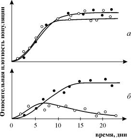
Rice. 9.3. A- Population growth curves of two species Parametium in single-species crops. Black circles – P Aurelia, white circles – P. Caudatum
b- Growth curves of P Aurelia and P . Caudatum in a mixed culture.
By Gause, 1934
The competition model (9.2) has disadvantages, in particular, it follows that the coexistence of two species is possible only if their numbers are limited by different factors, but the model does not indicate how large the differences must be to ensure long-term coexistence. At the same time, it is known that for long-term coexistence in a changing environment, a difference reaching a certain magnitude is necessary. Introducing stochastic elements into the model (for example, introducing a resource use function) allows us to quantitatively investigate these issues.
PREDATOR+VICTIM system
 (9.7)
(9.7)
Here, in contrast to (9.2), the signs b 12 And b 21 are different. As in the case of competition, the origin
![]() (9.8)
(9.8)
is a special point of the unstable node type. Three other possible steady states:
![]() ,(9.9)
,(9.9)
![]() (9.10)
(9.10)
![]() (9.11)
(9.11)
Thus, it is possible for only the prey to survive (9.10), only the predator (9.9) (if it has other food sources) and the coexistence of both species (9.11). We have already discussed the last option in Lecture 5. Possible types of phase portraits for a predator-prey system are presented in Fig. 9.4.
Isoclins of horizontal tangents are straight lines
x 2 = – b 21 X 1 /c 2 + a 1/c 2, X 2 = 0,
and isoclines of vertical tangents– straight
x 2 = – c 1 X 1 /b 12 + a 2 /b 12 , X 1 = 0.
Stationary points lie at the intersection of vertical and horizontal tangent isoclines.

From Fig. 9.4 the following is visible. Predator-prey system (9.7) can have a stable equilibrium position, in which o Rum population of victims completely died out ( ) and only predators remained (period 2 in Fig. 9.4 A). Obviously, such a situation can only be realized if, in addition to the type of victims in question, X 1 predator X 2 – has additional power sources. This fact is reflected in the model by the positive term on the right side of the equation for x2. Special points(1) and (3) (Fig. 9.4 A) are unstable. Second possibility – a stable stationary state in which the population of predators has completely died out and only prey remains – stable point(3) (Fig. 9.4 6 ). This is a special point (1) – also an unstable node.
Finally, the third possibility – sustainable coexistence of predator and prey populations (Fig. 9.4 V), the stationary numbers of which are expressed by the formulas (9.11).
As in the case of one population (see Lecture 3), for the model (9.7) It is possible to develop a stochastic model, but it cannot be solved explicitly. Therefore, we will limit ourselves to general considerations. Let us assume, for example, that the equilibrium point is located at a certain distance from each of the axes. Then for phase trajectories on which the valuesx 1 , x 2 remain large enough, a deterministic model will be quite satisfactory. But if at some point in the phase trajectory any variable is not very large, then random fluctuations can become significant. They lead to the fact that the representing point moves to one of the axes, which means the extinction of the corresponding species.
Thus, the stochastic model turns out to be unstable, since the stochastic “drift” sooner or later leads to the extinction of one of the species. In this kind of model, the predator eventually goes extinct, either by chance or because its prey population is eliminated first. The stochastic model of the predator-prey system explains Gause’s experiments well (Gause, 1934), in which ciliates Paramettum candatum served as a victim for another ciliate Didinium nasatum – predator. Expected according to deterministic equations (9.7) the equilibrium numbers in these experiments were approximately only five individuals of each species, so it is not surprising that in each repeated experiment either the predators or the prey (and after them the predators) died out quite quickly. The results of the experiments are presented in Fig. 9.5.

Rice. 9.5. Height Parametium caudatum and predatory ciliates Dadinium nasutum. From : Gause G.F. The struggle for existence. Baltimore, 1934
So, the analysis of Volterra models of species interaction shows that, despite the wide variety of types of behavior of such systems, there cannot be undamped fluctuations in numbers in the model of competing species at all. However, such oscillations are observed in nature and in experiment. The need for their theoretical explanation was one of the reasons for formulating model descriptions in a more general form.
Generalized models of interaction of two types
A large number of models have been proposed to describe the interaction of species, the right-hand sides of the equations of which were functions of the numbers of interacting populations. The issue of developing general criteria to establish what type of functions can describe the behavior of the temporary population size, including stable fluctuations, was resolved. The most famous of these models belong to Kolmogorov (1935, revised article - 1972) and Rosenzweig (1963).
 (9.12)
The model includes the following assumptions:
1) Predators do not interact with each other, i.e. predator reproduction rate k 2 and number of victims L exterminated per unit time by one predator does not depend on y.
2) The increase in the number of prey in the presence of predators is equal to the increase in the absence of predators minus the number of prey exterminated by predators. Functions k 1 (x), k 2 (x), L(x), are continuous and defined on the positive semi-axis x, y³ 0.
3) dk 1 /dx< 0. This means that the reproduction rate of prey in the absence of a predator decreases monotonically with an increase in the number of prey, which reflects the limited availability of food and other resources.
4) dk 2 /dx> 0, k 2 (0) < 0 < k 2 (¥ ). With an increase in the number of prey, the reproduction coefficient of predators decreases monotonically with an increase in the number of prey, moving from negative values, (when there is nothing to eat) to positive.
5) The number of prey destroyed by one predator per unit of time L(x)> 0 at N> 0; L(0)=0.
Possible types of phase portraits of system (9.12) are presented in Fig. 9.6:

Rice. 9.6.Phase portraits of the Kolmogorov system (9.12), which describes the interaction of two types at different ratios of parameters. Explanations in the text.
Stationary solutions (there are two or three) have the following coordinates:
(1). ` x=0;` y=0.
The origin of coordinates for any parameter values is a saddle (Fig. 9.6 a-d).
(2). ` x=A,` y=0.(9.13)
Adetermined from the equation:
k 1 (A)=0.
Stationary solution (9.13) is a saddle if B< A (Fig. 9.6 A, b, G), B determined from the equation
k 2 (B)=0
Point (9.13) is placed in the positive quadrant if B>A . This is a stable node .
The last case, which corresponds to the death of the predator and the survival of the prey, is shown in Fig. 9.6 V.
(3). ` x=B,` y=C.(9.14)
The value of C is determined from the equations:
Point (9.14) – focus (Fig.9.6 A) or node (Fig.9.6 G), the stability of which depends on the sign of the quantitys
s 2 = – k 1 (B) – k 1 (B)B+L(B)C.
If s>0, a point is stable ifs<0 ‑ точка неустойчива, и вокруг нее могут существовать предельные циклы (рис. 9.6 b)
In foreign literature, a similar model proposed by Rosenzweig and MacArthur (1963) is more often considered:
 (9.15)
Where f(x) - rate of change in the number of victims x in the absence of predators, F( x,y) - intensity of predation, k- coefficient characterizing the efficiency of processing prey biomass into predator biomass, e- predator mortality.
Model (9.15) reduces to a special case of the Kolmogorov model (9.12) under the following assumptions:
1) the number of predators is limited only by the number of prey,
2) the speed with which a given predator eats prey depends only on the density of the prey population and does not depend on the density of the predator population.
Then equations (9.15) take the form.

When describing the interaction of real species, the right-hand sides of the equations are specified in accordance with ideas about biological realities. Let's consider one of the most popular models of this type.
Model of interaction between two types of insects (MacArthur, 1971)
The model, which we will consider below, was used to solve the practical problem of controlling harmful insects by sterilizing the males of one of the species. Based on the biological features of species interaction, the following model was written
 (9.16)
Here x,y- biomass of two types of insects. The trophic interactions of the species described in this model are very complex. This determines the form of polynomials on the right-hand sides of the equations.
Let's look at the right side of the first equation. Insect species X eat the larvae of the species at(member +k 3 y), but adults of the species at eat the larvae of the species X subject to high species abundance X or at or both types (members –k 4 xy, – y 2). At small X species mortality X higher than its natural increase (1 –k 1 +k 2 x–x 2 < 0 at small X). In the second equation the term k 5 reflects the natural growth of the species y; –k 6 y – self-restraint of this type,–k 7 x– eating larvae of the species at insect species x, k 8 xy – increase in species biomass at due to consumption by adult insects of the species at larvae of the species X.
In Fig. 9.7 a limit cycle is presented, which is the trajectory of a stable periodic solution of the system (9.16).

The solution to the question of how to ensure the coexistence of a population with its biological environment, of course, cannot be obtained without taking into account the specifics of a particular biological system and an analysis of all its interrelations. At the same time, the study of formal mathematical models allows us to answer some general questions. It can be argued that for models like (9.12), the fact of compatibility or incompatibility of populations does not depend on their initial size, but is determined only by the nature of the interaction of species. The model helps answer the question: how to influence the biocenosis and manage it in order to quickly destroy the harmful species.
Management can be reduced to a short-term, abrupt change in population values X And u. This method corresponds to control methods such as the one-time destruction of one or both populations by chemical means. From the statement formulated above it is clear that for compatible populations this method of control will be ineffective, since over time the system will again reach a stationary regime.
Another way is to change the type of interaction functions between views, for example, when changing the values of system parameters. It is this parametric method that biological control methods correspond to. Thus, when sterilized males are introduced, the rate of natural population growth decreases. If at the same time we get a different type of phase portrait, one where there is only a stable stationary state with zero pest numbers, the control will lead to the desired result – destruction of the population of a harmful species. It is interesting to note that sometimes it is advisable to apply the impact not to the pest itself, but to its partner. In general, it is impossible to say which method is more effective. This depends on the controls available and on the explicit form of the functions describing the interaction of populations.
Model by A.D. Bazykin
The theoretical analysis of models of species interactions was most comprehensively carried out in A.D. Bazykin’s book “Biophysics of Interacting Populations” (M., Nauka, 1985).
Let's consider one of the predator-prey models studied in this book.
 (9.17)
System (9.17) is a generalization of the simplest Volterra predator-prey model (5.17) taking into account the effect of predator saturation. Model (5.17) assumes that the intensity of prey grazing increases linearly with increasing prey density, which does not correspond to reality at high prey densities. Different functions can be chosen to describe the dependence of a predator's diet on prey density. It is most important that the chosen function with growth x tended asymptotically to a constant value. Model (9.6) used a logistic dependence. In Bazykin’s model, the hyperbola is chosen as such a function x/(1+px). Let us remember that this is the form of the Monod formula, which describes the dependence of the growth rate of microorganisms on the concentration of the substrate. Here the prey plays the role of the substrate, and the predator plays the role of microorganisms. .
System (9.17) depends on seven parameters. The number of parameters can be reduced by replacing variables:
x® (A/D)x; y ® (A/D)/y;
t® (1/A)t; g (9.18)
and depends on four parameters.
For a complete qualitative study, it is necessary to divide the four-dimensional parameter space into areas with different types of dynamic behavior, i.e. build a parametric or structural portrait of the system.
Then it is necessary to construct phase portraits for each of the areas of the parametric portrait and describe the bifurcations that occur with the phase portraits at the boundaries of different areas of the parametric portrait.
The construction of a complete parametric portrait is carried out in the form of a set of “slices” (projections) of a low-dimensional parametric portrait with fixed values of some of the parameters.
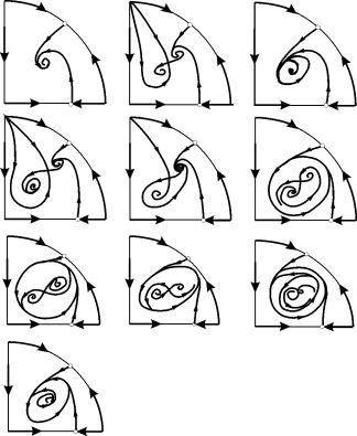
Parametric portrait of system (9.18) for fixed g and small e presented in Fig. 9.8. The portrait contains 10 areas with different types of behavior of phase trajectories.
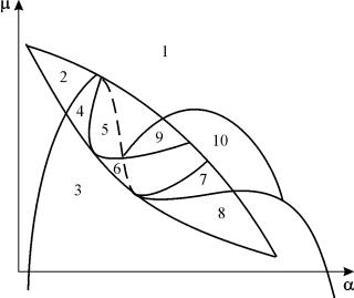
Rice. 9.8.Parametric portrait of system (9.18) for fixedg
and small e
The behavior of the system at different ratios of parameters can be significantly different (Fig. 9.9). The system allows:
1) one stable equilibrium (regions 1 and 5);
2) one stable limit cycle (regions 3 and 8);
3) two stable equilibria (region 2)
4) stable limit cycle and unstable equilibrium inside it (regions 6, 7, 9, 10)
5) stable limit cycle and stable equilibrium outside it (region 4).
In parametric regions 7, 9, 10, the region of attraction of equilibrium is limited by an unstable limit cycle lying inside a stable one. The most interesting structure is the phase portrait, corresponding to area 6 in the parametric portrait. It is shown in detail in Fig. 9.10.
The area of attraction of equilibrium B 2 (shaded) is a “snail” twisting from the unstable focus B 1. If it is known that at the initial moment of time the system was in the neighborhood of B 1, then it is possible to judge whether the corresponding trajectory will reach equilibrium B 2 or a stable limit cycle surrounding three equilibrium points C (saddle), B 1 and B 2 based on probabilistic considerations.
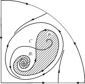
Fig.9.10.Phase portrait of system 9.18 for parametric region 6. Attraction region B 2 is shaded
In a parametric portrait(9.7) there are 22 various bifurcation boundaries that form 7 various types of bifurcations. Their study allows us to identify possible types of system behavior when its parameters change. For example, when moving from the area 1 to area 3 the birth of a small limit cycle occurs, or the soft birth of self-oscillations around a single equilibrium IN. A similar soft birth of self-oscillations, but around one of the equilibria, namely B 1 , occurs when crossing the boundaries of regions 2 and 4. When leaving the area 4 to area 5 stable limit cycle around a pointB 1 “bursts” on the loop of separatrices and the only attracting point remains equilibrium B 2 etc.
Of particular interest for practice is, of course, the development of criteria for the proximity of a system to bifurcation boundaries. Indeed, biologists are well aware of the “buffering” or “flexibility” property of natural ecological systems. These terms usually refer to the ability of a system to absorb external influences. As long as the intensity of the external influence does not exceed a certain critical value, the behavior of the system does not undergo qualitative changes. On the phase plane, this corresponds to the return of the system to a stable state of equilibrium or to a stable limit cycle, the parameters of which do not differ much from the original one. When the intensity of the impact exceeds the permissible level, the system “breaks down” and goes into a qualitatively different mode of dynamic behavior, for example, it simply dies out. This phenomenon corresponds to a bifurcation transition.
Each type of bifurcation transition has its own distinctive features, which make it possible to judge the danger of such a transition for the ecosystem. Here are some general criteria indicating the proximity of a dangerous border. As in the case of one species, if, when the number of one of the species decreases, the system “gets stuck” near an unstable saddle point, which is expressed in a very slow restoration of the number to the initial value, then the system is near the critical boundary. An indicator of danger is also a change in the shape of fluctuations in the numbers of predator and prey. If oscillations that are close to harmonic become relaxation ones, and the amplitude of the oscillations increases, this can lead to a loss of stability of the system and the extinction of one of the species.
Further deepening of the mathematical theory of interaction between species goes along the lines of detailing the structure of the populations themselves and taking into account temporal and spatial factors.
Literature.
Kolmogorov A.N. Qualitative study of mathematical models of population dynamics. // Problems of cybernetics. M., 1972, Issue 5.
MacArtur R. Graphical analysis of ecological systems // Division of biology report Perinceton University. 1971
A.D. Bazykin “Biophysics of interacting populations.” M., Nauka, 1985.
V. Volterra: “Mathematical theory of the struggle for existence.” M.. Science, 1976
Gause G.F. The struggle for existence. Baltimore, 1934.